How to use MicrogliaMorphologyR
MicrogliaMorphologyR.RmdYou can read more about any of the MicrogliaMorphologyR functions covered in this tutorial by calling to their respective help pages by running ?function_name in the console.
Load in MicrogliaMorphology ImageJ macro output and explore data
Load packages and set seed for reproducibility of results shown here
library(MicrogliaMorphologyR)
library(factoextra)
library(ppclust)
set.seed(1)We will start by loading in your MicrogliaMorphology output (FracLac
and SkeletonAnalysis files) and formatting the data using the
metadata_columns function so that you have a final
dataframe which contains your cell-level data, with every row as a
single cell and every column as either a metadata descriptor or
morphology measure. The metadata_columns function relies on
each piece of metadata to be separated by a common deliminator such as
“_” or “-” in the “Name” column. You can read more about the function by
calling to its help page using ?metadata_columns
Load in your fraclac and skeleton data, tidy, and merge into final data frame
fraclac.dir <- "insert path to fraclac directory"
skeleton.dir <- "insert path to skeleton analysis directory"

# these steps may be very time-intensive, depending on how many cells you are analyzing (i.e., on the order of 1000s of cells).
fraclac <- fraclac_tidying(fraclac.dir)
skeleton <- skeleton_tidying(skeleton.dir)

data <- merge_data(fraclac, skeleton)
finaldata <- metadata_columns(data, c("Antibody","Paper","Cohort","MouseID","Sex","Treatment","BrainRegion","Subregion"), sep="_")
For demonstration purposes, we will use one of the datasets that comes packaged with MicrogliaMorphologyR. ‘data_2xLPS_mouse’ contains morphology data collected from female and male 8 week-old Cx3cr1-eGFP mice, which were given 2 i.p. injections of either PBS vehicle solution or 0.5mg/kg lipopolysaccharides (LPS), spaced 24 hours apart. In this genetic mouse line, Cx3cr1-expressing cells including microglia have an endogenous reporter which makes them green when immunofluorescently imaged. Brains were collected 3 hours after the final injections, and brain sections were immunofluorescently stained and imaged for 2 additional, commonly used microglia markers: P2ry12, and Iba1.
Load in example dataset
data_2xLPS <- MicrogliaMorphologyR::data_2xLPS_mouseGenerate heatmap of correlations across features
We start by exploring the morphology features measured by MicrogliaMorphology and how they relate to each other by generating a heatmap of spearman’s correlations across the 27 different morphology features. As expected, the features which describe similar aspects of morphology are more highly correlated to each other than to other features which do not. For example, the numbers of end point voxels, junction voxels, triple points, branches, and junctions all explain cell branching complexity and are highly correlated to each other.
featurecorrelations(data_2xLPS,
                    featurestart=9, featureend=35,
                    rthresh=0.8, pthresh=0.05,
                    title="Correlations across features")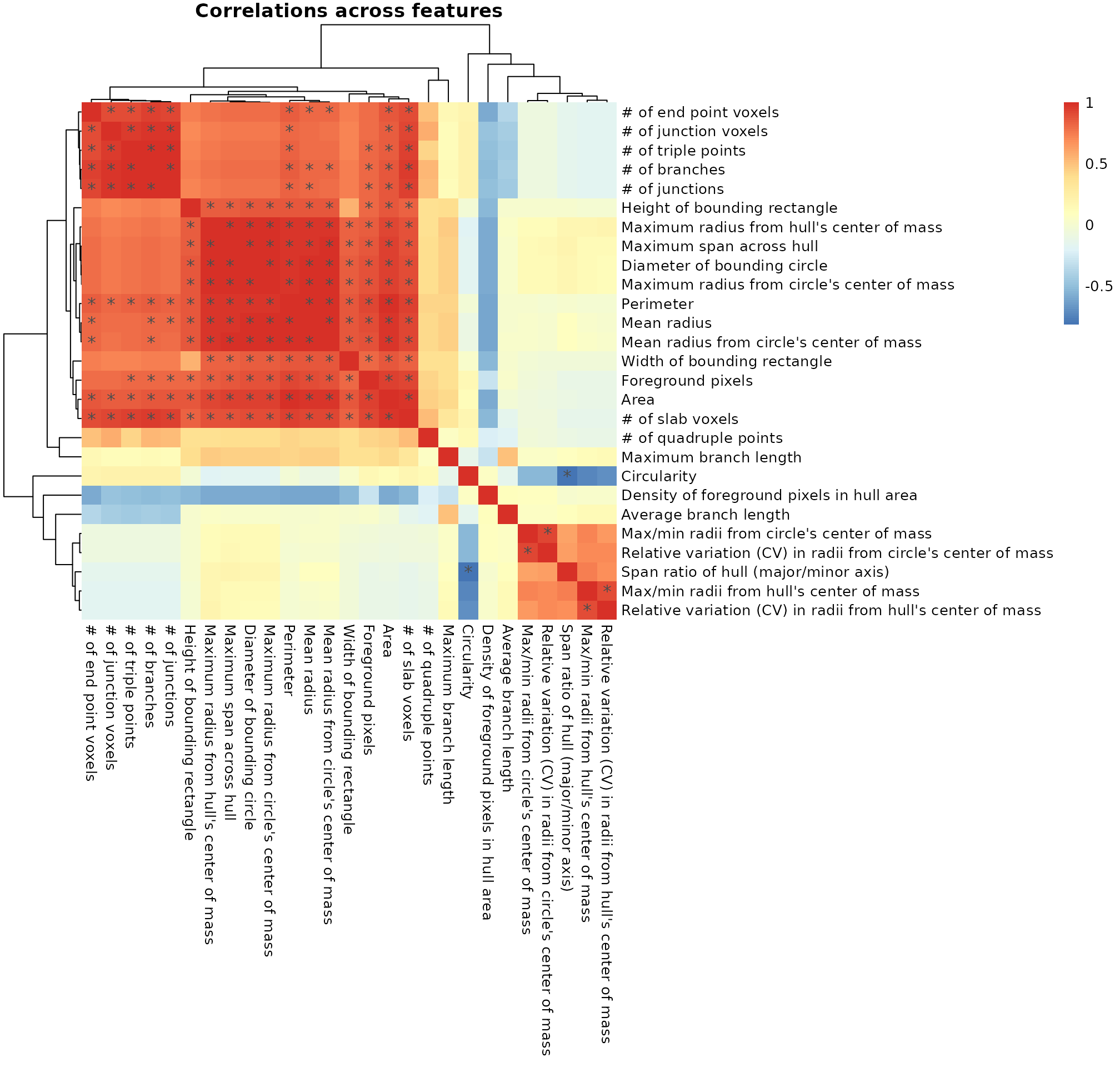
# to get the underlying stats depicted in the heatmap above
correlationstats <- featurecorrelations_stats(data_2xLPS,
                                             featurestart=9, featureend=35,
                                             rthresh=0.8, pthresh=0.05)
correlationstats %>% head()
#>       measure_a             measure_b correlation pvalues Significant
#> 1 # of branches         # of branches   1.0000000      NA        <NA>
#> 2 # of branches # of end point voxels   0.9425514       0 significant
#> 3 # of branches  # of junction voxels   0.9757485       0 significant
#> 4 # of branches        # of junctions   0.9970174       0 significant
#> 5 # of branches # of quadruple points   0.5349538       0          ns
#> 6 # of branches      # of slab voxels   0.9464104       0 significant
MicrogliaMorphologyR comes with a number of functions which allow you to explore which features have extreme outliers and how normalizing in various ways changes your feature distributions. This allows you to explore and transform your data in a dataset-appropriate manner for downstream analyses. In later steps, we will be running Principal Components Analysis (PCA) on our transformed data. PCA is a statistical technique which identifies the most significant variables and relationships in your data, and can be used as a pre-processing step to reduce noise and remove irrelevant features to improve the efficiency and accuracy of downstream analysis. PCA assumes that the variables in your dataset follow a normal distribution, and violations of normality can affect the accuracy of PCA results. Thus, it is important to transform your data so that the distributions of the values for each individual morphology measure approximate normality as much as possible.
The morphology features measured using MicrogliaMorphology are often suitable for PCA after log transformation. Because many of the measures contain zero values (e.g., numbers of junctions, numbers of branches, etc.), we need to add a constant to our data prior to log transforming.
Exploratory data visualization and data transformation for downstream analyses
# gather your numerical morphology data into one column ('measure') which contains the feature name, and another column ('value') which contains measured values
data_2xLPS_gathered <- data_2xLPS %>% gather(measure, value, 9:ncol(data_2xLPS))

# check for outliers
outliers_boxplots(data_2xLPS_gathered)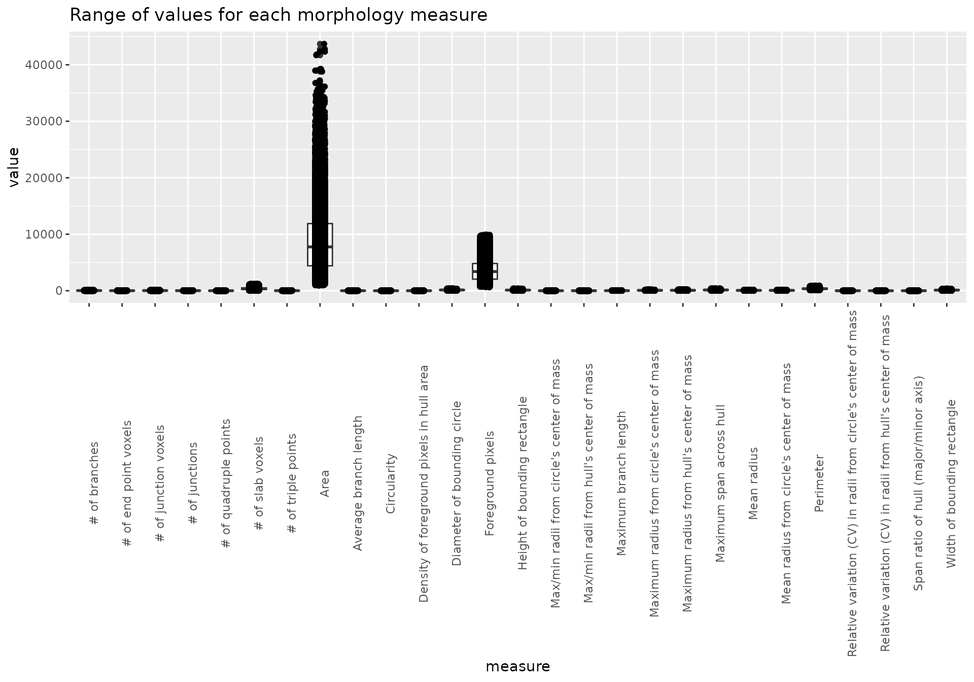
outliers_distributions(data_2xLPS_gathered)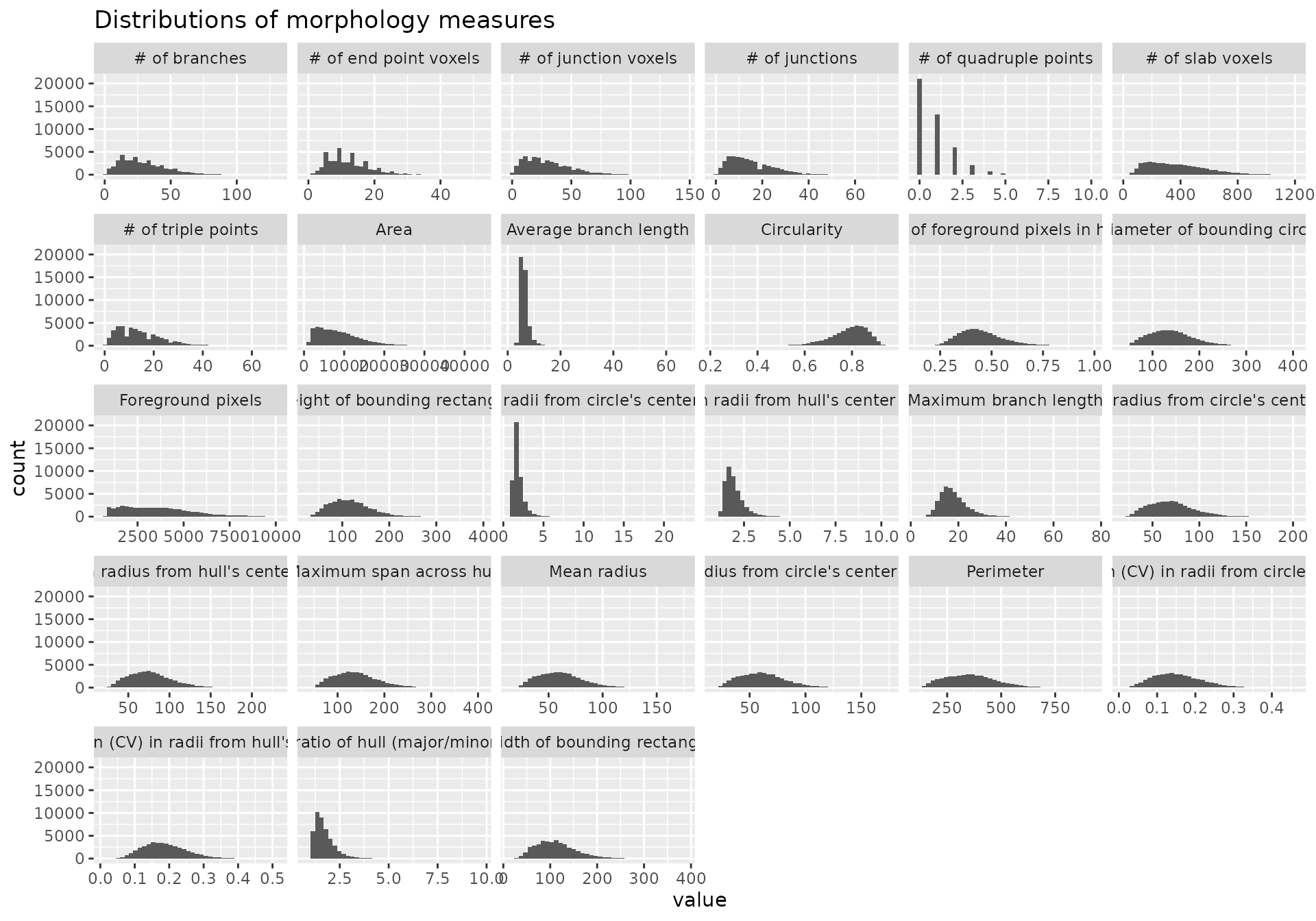
# checking different normalization features
normalize_logplots(data_2xLPS_gathered,1)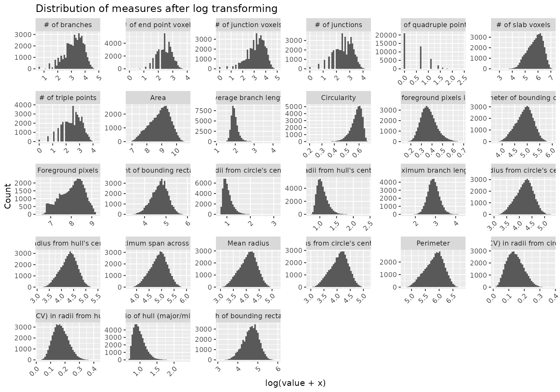
normalize_minmax(data_2xLPS_gathered)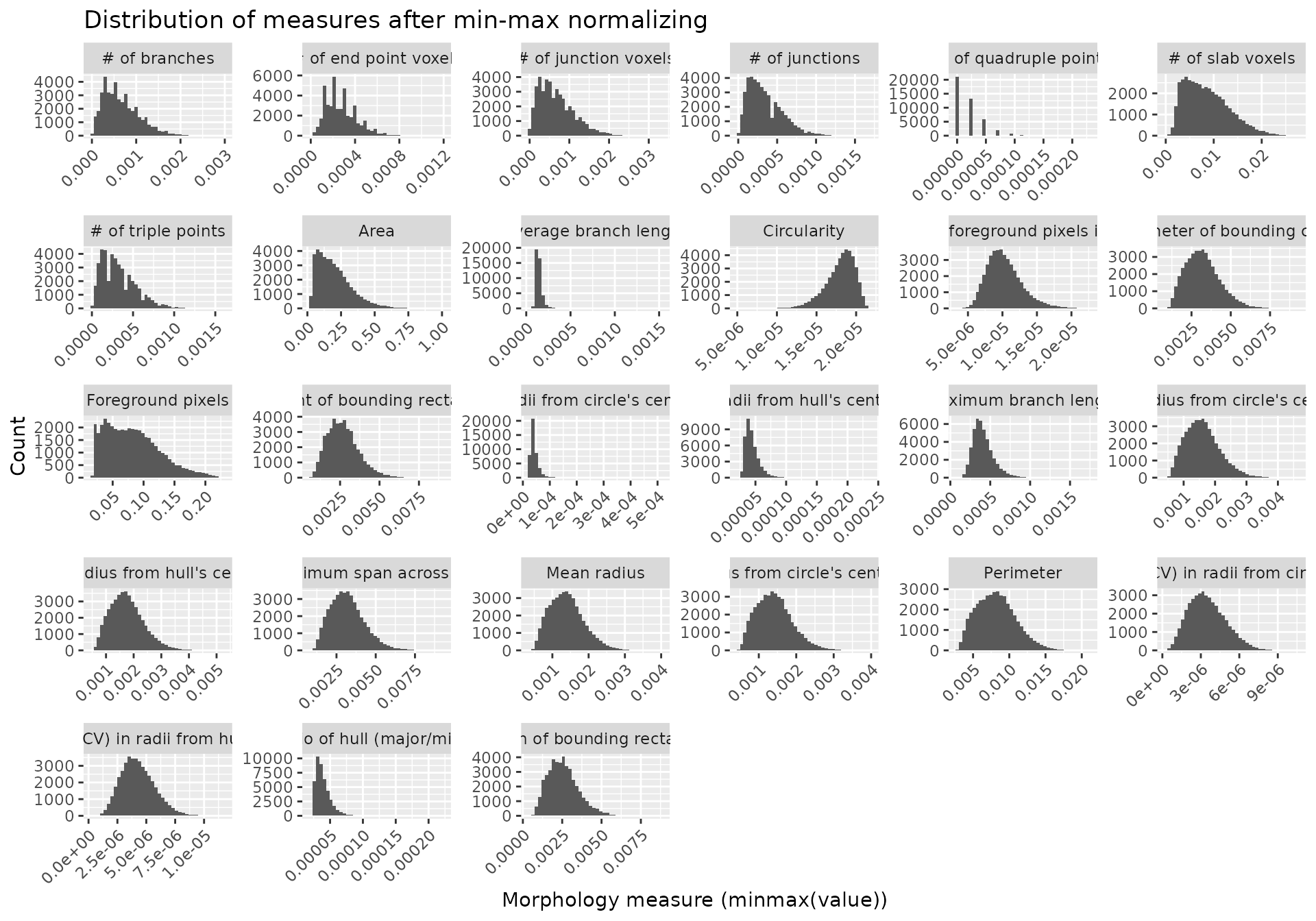
normalize_scaled(data_2xLPS_gathered)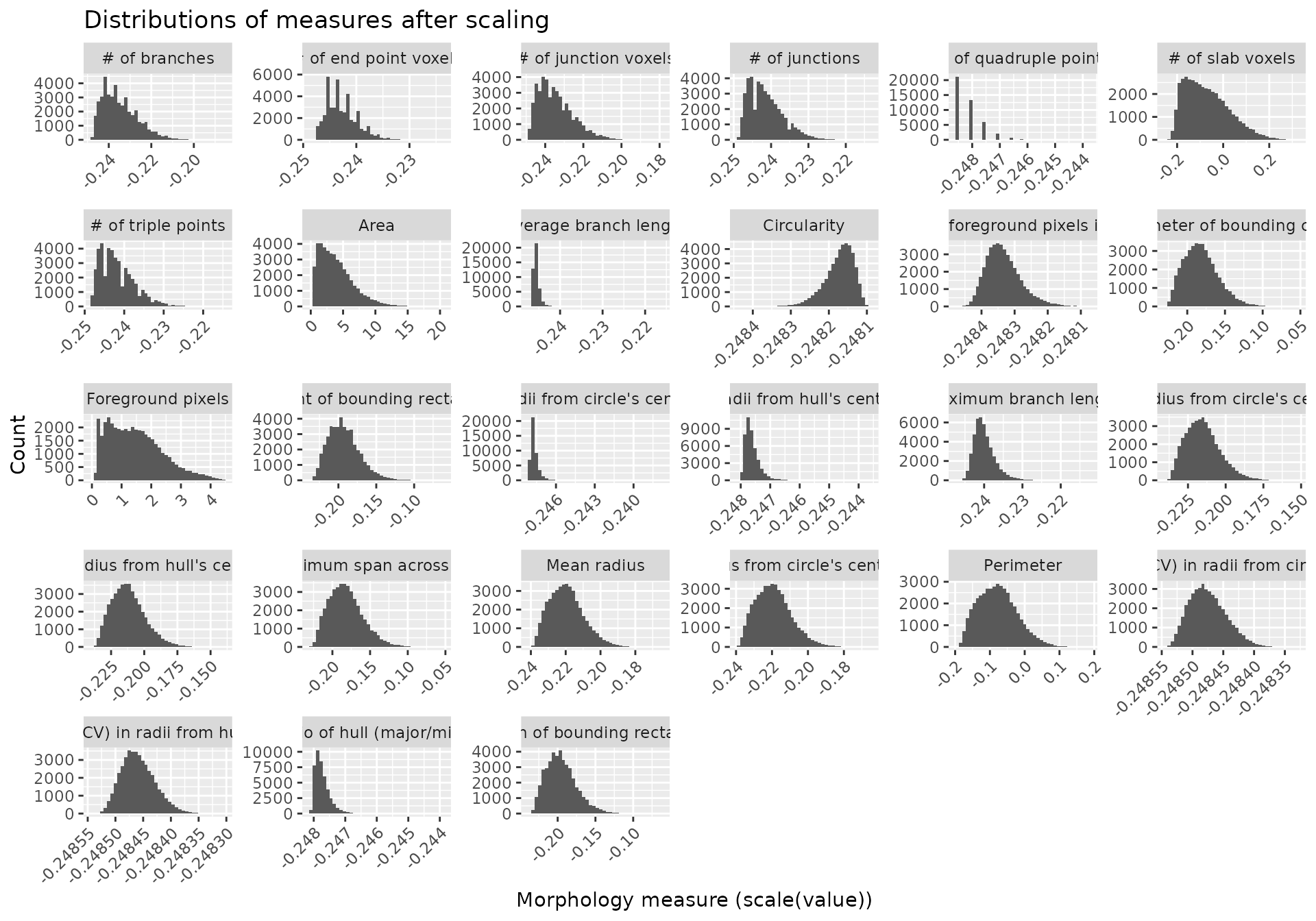
# transform your data in appropriate manner for downstream analyses
# we will use the logtransformed data as our PCA input
data_2xLPS_logtransformed <- transform_log(data_2xLPS, 1, start=9, end=35)
data_2xLPS_minmaxtransformed <- transform_minmax(data_2xLPS, start=9, end=35)
data_2xLPS_scaled <- transform_scale(data_2xLPS, start=9, end=35)

# get sample size of data based on factors of interest
samplesize(data_2xLPS, MouseID, Antibody)
#> # A tibble: 18 × 3
#> # Groups:   MouseID [6]
#>    MouseID Antibody   num
#>    <chr>   <chr>    <int>
#>  1 1       Cx3cr1    1703
#>  2 1       Iba1      1737
#>  3 1       P2ry12    2105
#>  4 2       Cx3cr1    2496
#>  5 2       Iba1      2927
#>  6 2       P2ry12    4341
#>  7 3       Cx3cr1    1145
#>  8 3       Iba1      1310
#>  9 3       P2ry12    1978
#> 10 4       Cx3cr1    1775
#> 11 4       Iba1      2044
#> 12 4       P2ry12    2372
#> 13 5       Cx3cr1    2053
#> 14 5       Iba1      2302
#> 15 5       P2ry12    3513
#> 16 6       Cx3cr1    2771
#> 17 6       Iba1      3095
#> 18 6       P2ry12    3665
samplesize(data_2xLPS, Sex, Treatment, Antibody)
#> # A tibble: 12 × 4
#> # Groups:   Sex, Treatment [4]
#>    Sex   Treatment Antibody   num
#>    <chr> <chr>     <chr>    <int>
#>  1 F     2xLPS     Cx3cr1    3478
#>  2 F     2xLPS     Iba1      3781
#>  3 F     2xLPS     P2ry12    4477
#>  4 F     PBS       Cx3cr1    3641
#>  5 F     PBS       Iba1      4237
#>  6 F     PBS       P2ry12    6319
#>  7 M     2xLPS     Cx3cr1    2771
#>  8 M     2xLPS     Iba1      3095
#>  9 M     2xLPS     P2ry12    3665
#> 10 M     PBS       Cx3cr1    2053
#> 11 M     PBS       Iba1      2302
#> 12 M     PBS       P2ry12    3513
Obtain density measures for each image (using Areas.csv file output from MicrogliaMorphology)
Note: The areas obtained in this file are dataset-specific and will be in the units of your original input images
# list out all variables of interest present in the original image names to obtain numbers of microglia per image
microglianumbers <- samplesize(data_2xLPS, Antibody, MouseID, Sex, Treatment, BrainRegion, Subregion)
microglianumbers %>% print(n=3, width=Inf)
#> # A tibble: 148 × 7
#> # Groups:   Antibody, MouseID, Sex, Treatment, BrainRegion [51]
#>   Antibody MouseID Sex   Treatment BrainRegion Subregion   num
#>   <chr>    <chr>   <chr> <chr>     <chr>       <chr>     <int>
#> 1 Cx3cr1   1       F     2xLPS     FC          ACC          93
#> 2 Cx3cr1   1       F     2xLPS     FC          IL          161
#> 3 Cx3cr1   1       F     2xLPS     FC          PL          112
#> # ℹ 145 more rows

# add Name column back in -- make sure that the resulting strings in the Name column match the names of your original input .tiff files that you used for MicrogliaMorphology !!
microglianumbers <- microglianumbers %>% unite("Name", Antibody:Subregion, sep="_", remove=FALSE)
microglianumbers %>% print(n=3, width=Inf)
#> # A tibble: 148 × 8
#> # Groups:   Antibody, MouseID, Sex, Treatment, BrainRegion [51]
#>   Name                    Antibody MouseID Sex   Treatment BrainRegion Subregion
#>   <chr>                   <chr>    <chr>   <chr> <chr>     <chr>       <chr>
#> 1 Cx3cr1_1_F_2xLPS_FC_ACC Cx3cr1   1       F     2xLPS     FC          ACC
#> 2 Cx3cr1_1_F_2xLPS_FC_IL  Cx3cr1   1       F     2xLPS     FC          IL
#> 3 Cx3cr1_1_F_2xLPS_FC_PL  Cx3cr1   1       F     2xLPS     FC          PL
#>     num
#>   <int>
#> 1    93
#> 2   161
#> 3   112
#> # ℹ 145 more rows

# path to Areas.csv file
AreasPath <- "./man/data/Areas.csv"

# use celldensity function to calculate density at image-level: values are under the "Density" column
Density <- celldensity(AreasPath, microglianumbers)
#> Warning: Expected 2 pieces. Additional pieces discarded in 148 rows [1, 2, 3, 4, 5, 6,
#> 7, 8, 9, 10, 11, 12, 13, 14, 15, 16, 17, 18, 19, 20, ...].
Density %>% print(n=5, width=Inf)
#> # A tibble: 148 × 10
#> # Groups:   Antibody, MouseID, Sex, Treatment, BrainRegion [51]
#>   Name                    Antibody MouseID Sex   Treatment BrainRegion Subregion
#>   <chr>                   <chr>    <chr>   <chr> <chr>     <chr>       <chr>
#> 1 Cx3cr1_1_F_2xLPS_FC_ACC Cx3cr1   1       F     2xLPS     FC          ACC
#> 2 Cx3cr1_1_F_2xLPS_FC_IL  Cx3cr1   1       F     2xLPS     FC          IL
#> 3 Cx3cr1_1_F_2xLPS_FC_PL  Cx3cr1   1       F     2xLPS     FC          PL
#> 4 Cx3cr1_1_F_2xLPS_HC_CA1 Cx3cr1   1       F     2xLPS     HC          CA1
#> 5 Cx3cr1_1_F_2xLPS_HC_CA2 Cx3cr1   1       F     2xLPS     HC          CA2
#>     num     Area  Density
#>   <int>    <dbl>    <dbl>
#> 1    93  333722. 0.000279
#> 2   161  589983. 0.000273
#> 3   112  423038. 0.000265
#> 4   263 1018060. 0.000258
#> 5    43  172581. 0.000249
#> # ℹ 143 more rows
if you want to group on another variable, and then recalculate density
e.g., calculating density at the brain region-level rather than the subregion level (which are what the image rois capture in our example dataset)
Density %>%
  group_by(Antibody, MouseID, Sex, Treatment, BrainRegion) %>%
  summarise(num=sum(num), Area=sum(Area)) %>% # calculate new cell numbers and new areas at the brain region level
  mutate(Density=num/Area) # calculate new density at the brain region level
#> `summarise()` has grouped output by 'Antibody', 'MouseID', 'Sex', 'Treatment'.
#> You can override using the `.groups` argument.
#> # A tibble: 51 × 8
#> # Groups:   Antibody, MouseID, Sex, Treatment [18]
#>    Antibody MouseID Sex   Treatment BrainRegion   num     Area  Density
#>    <chr>    <chr>   <chr> <chr>     <chr>       <int>    <dbl>    <dbl>
#>  1 Cx3cr1   1       F     2xLPS     FC            366 1346743. 0.000272
#>  2 Cx3cr1   1       F     2xLPS     HC            723 2705033. 0.000267
#>  3 Cx3cr1   1       F     2xLPS     STR           614 2229707. 0.000275
#>  4 Cx3cr1   2       F     PBS       FC            523 1758434. 0.000297
#>  5 Cx3cr1   2       F     PBS       HC            667 2448885. 0.000272
#>  6 Cx3cr1   2       F     PBS       STR          1306 4608609. 0.000283
#>  7 Cx3cr1   3       F     PBS       FC            412 1496417. 0.000275
#>  8 Cx3cr1   3       F     PBS       STR           733 2624917. 0.000279
#>  9 Cx3cr1   4       F     2xLPS     FC            375 1762321. 0.000213
#> 10 Cx3cr1   4       F     2xLPS     HC            503 2154789. 0.000233
#> # ℹ 41 more rows
Now, since we have gotten a better feel for our data and how to transform it, we can proceed with PCA for dimensionality reduction and downstream clustering. We can see here that the first 3 PCs describe around ~85% of our data. We can also explore how each PC correlates to the 27 different morphology features to get a better understanding of how each PC describes the variability present in the data. This is useful to inform which to include for downstream clustering steps.
Dimensionality reduction using PCA
pcadata_elbow(data_2xLPS_logtransformed, featurestart=9, featureend=35)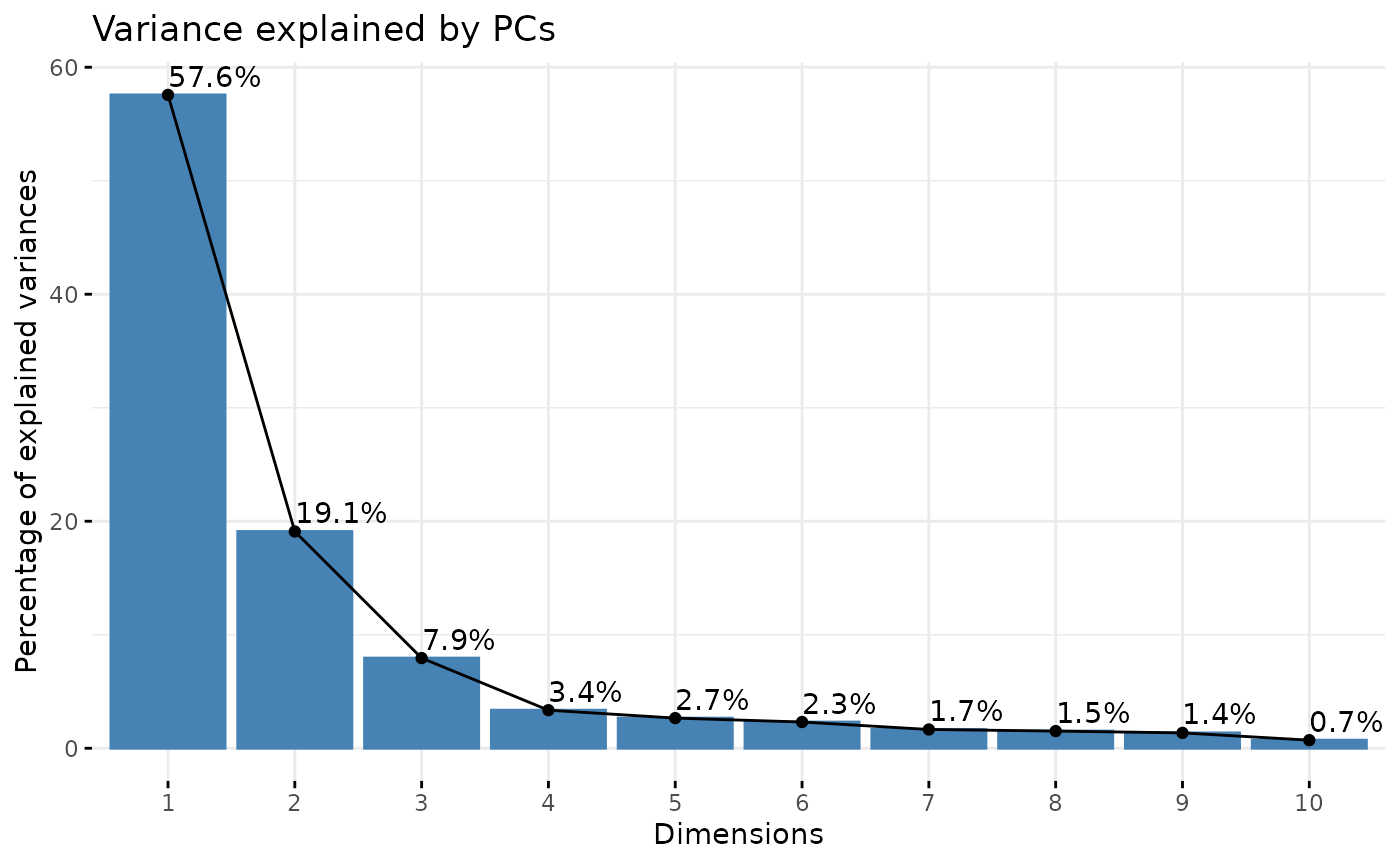
pca_data <- pcadata(data_2xLPS_logtransformed, featurestart=9, featureend=35,
                    pc.start=1, pc.end=10)
head(pca_data,3)
#>           PC1       PC2        PC3        PC4         PC5         PC6
#> 1 -3.40837468 0.6764322  2.4544974 -0.7011076  0.51923399  0.09841964
#> 2 -3.97236479 0.6876435 -0.1588262 -1.7816133 -0.29998161 -0.39435933
#> 3 -0.05205818 0.4984643  1.1106371 -1.7095791  0.05149981 -0.88502415
#>          PC7        PC8        PC9       PC10 Antibody MouseID Sex Treatment
#> 1 -0.1887577 -0.2217257 -1.4166585  0.7370713   Cx3cr1       1   F     2xLPS
#> 2 -0.4914042 -0.5946128  0.1761947 -0.2787745   Cx3cr1       1   F     2xLPS
#> 3 -0.1504321 -0.1952254 -0.6739042  0.3673300   Cx3cr1       1   F     2xLPS
#>   BrainRegion Subregion          ID
#> 1          FC       ACC 00002-01053
#> 2          FC       ACC 00009-01153
#> 3          FC       ACC 00015-01224
#>                                          UniqueID Foreground pixels
#> 1 Cx3cr1_Paper1_2Hit_1_F_2xLPS_FC_ACC_00002-01053          7.838343
#> 2 Cx3cr1_Paper1_2Hit_1_F_2xLPS_FC_ACC_00009-01153          7.837554
#> 3 Cx3cr1_Paper1_2Hit_1_F_2xLPS_FC_ACC_00015-01224          8.516593
#>   Density of foreground pixels in hull area
#> 1                                 0.4722511
#> 2                                 0.5270926
#> 3                                 0.5027128
#>   Span ratio of hull (major/minor axis) Maximum span across hull     Area
#> 1                             0.8187220                 4.516565 8.343078
#> 2                             0.9121221                 4.512384 8.202756
#> 3                             0.8887962                 4.867296 8.942330
#>   Perimeter Circularity Width of bounding rectangle
#> 1  5.579191   0.5642337                    4.406719
#> 2  5.458799   0.6092219                    4.219508
#> 3  5.863106   0.5771189                    4.682131
#>   Height of bounding rectangle Maximum radius from hull's center of mass
#> 1                     4.488636                                  3.945005
#> 2                     4.532599                                  3.927930
#> 3                     4.779123                                  4.213828
#>   Max/min radii from hull's center of mass
#> 1                                 1.017764
#> 2                                 1.085460
#> 3                                 1.044754
#>   Relative variation (CV) in radii from hull's center of mass Mean radius
#> 1                                                   0.1031882    3.833051
#> 2                                                   0.1719345    3.666266
#> 3                                                   0.1264564    4.100085
#>   Diameter of bounding circle Maximum radius from circle's center of mass
#> 1                    4.600622                                    3.917470
#> 2                    4.512384                                    3.830149
#> 3                    4.884708                                    4.199093
#>   Max/min radii from circle's center of mass
#> 1                                  0.9896899
#> 2                                  0.9603076
#> 3                                  0.9981288
#>   Relative variation (CV) in radii from circle's center of mass
#> 1                                                     0.1008403
#> 2                                                     0.1573456
#> 3                                                     0.1276013
#>   Mean radius from circle's center of mass # of branches # of junctions
#> 1                                 3.828354      2.564949       1.945910
#> 2                                 3.649437      2.708050       1.945910
#> 3                                 4.100996      3.135494       2.484907
#>   # of end point voxels # of junction voxels # of slab voxels
#> 1              1.945910             2.564949         5.484797
#> 2              2.302585             2.708050         5.342334
#> 3              2.397895             3.135494         5.846439
#>   Average branch length # of triple points # of quadruple points
#> 1              2.275111           1.945910             0.0000000
#> 2              2.044073           1.791759             0.6931472
#> 3              2.100836           2.397895             0.6931472
#>   Maximum branch length
#> 1              3.409033
#> 2              2.778384
#> 3              3.102836
Generate heatmap of correlations between PCs and features
Using the pcfeaturecorrelations function, we can
investigate the relationships of our 27 individual morphology measures
to the principle components to examine how each PC is differentially
correlated to and described by different sets of morphology features.
For example, we can see that PC1 is highly positively correlated to
features describing branching complexity and territory span, meaning
that individual cells with greater branching complexity or area have
higher PC1 scores in our dataset. Similarly, the variability in our
dataset represented in PC2 is described by cell shape: 1)
circularity (circularity, max/min radii from center, span ratio
of hull) and 2) branching homogeneity (relative variation (CV)
from center of mass), and PC3 is described by branch length-related
measures. Generally, you will see the same types of features describing
the first four PCs after dimensionality reduction, although the
directionality of the correlations could be inversed, which is normal as
long as the sets of features that are highly correlated (e.g.,
circularity and branching homogeneity for PC2) are still maintained.
pcfeaturecorrelations(pca_data, pc.start=1, pc.end=3,
                      feature.start=19, feature.end=45,
                      rthresh=0.75, pthresh=0.05,
                      title="Correlation between PCs and features")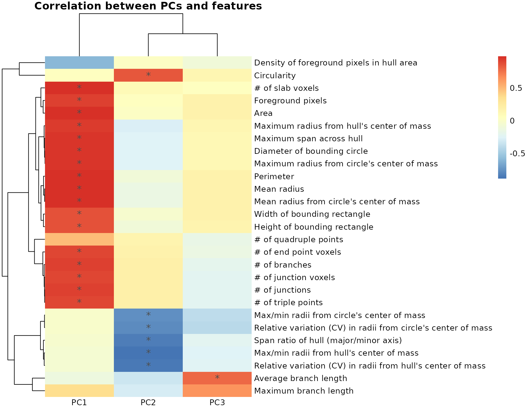
# to get the underlying stats depicted in the heatmap above
correlationstats <- pcfeaturecorrelations_stats(pca_data, pc.start=1, pc.end=3,
                                                feature.start=19, feature.end=45,
                                                rthresh=0.75, pthresh=0.05)
correlationstats %>% head()
#>               measure_a measure_b correlation pvalues Significant
#> 1         # of branches       PC1   0.9202371       0 significant
#> 2         # of branches       PC2   0.1922737       0          ns
#> 3         # of branches       PC3  -0.2115683       0          ns
#> 4 # of end point voxels       PC1   0.9063301       0 significant
#> 5 # of end point voxels       PC2   0.1644570       0          ns
#> 6 # of end point voxels       PC3  -0.1465995       0          ns
Visually explore different sources of variability in dataset
# gather your data by experimental variables (e.g., Treatment, Sex, MouseID, etc.)
gathered_expvariables <- pca_data %>% gather(variable, value, 11:16)

plots_expvariable(gathered_expvariables, "PC1", "PC2")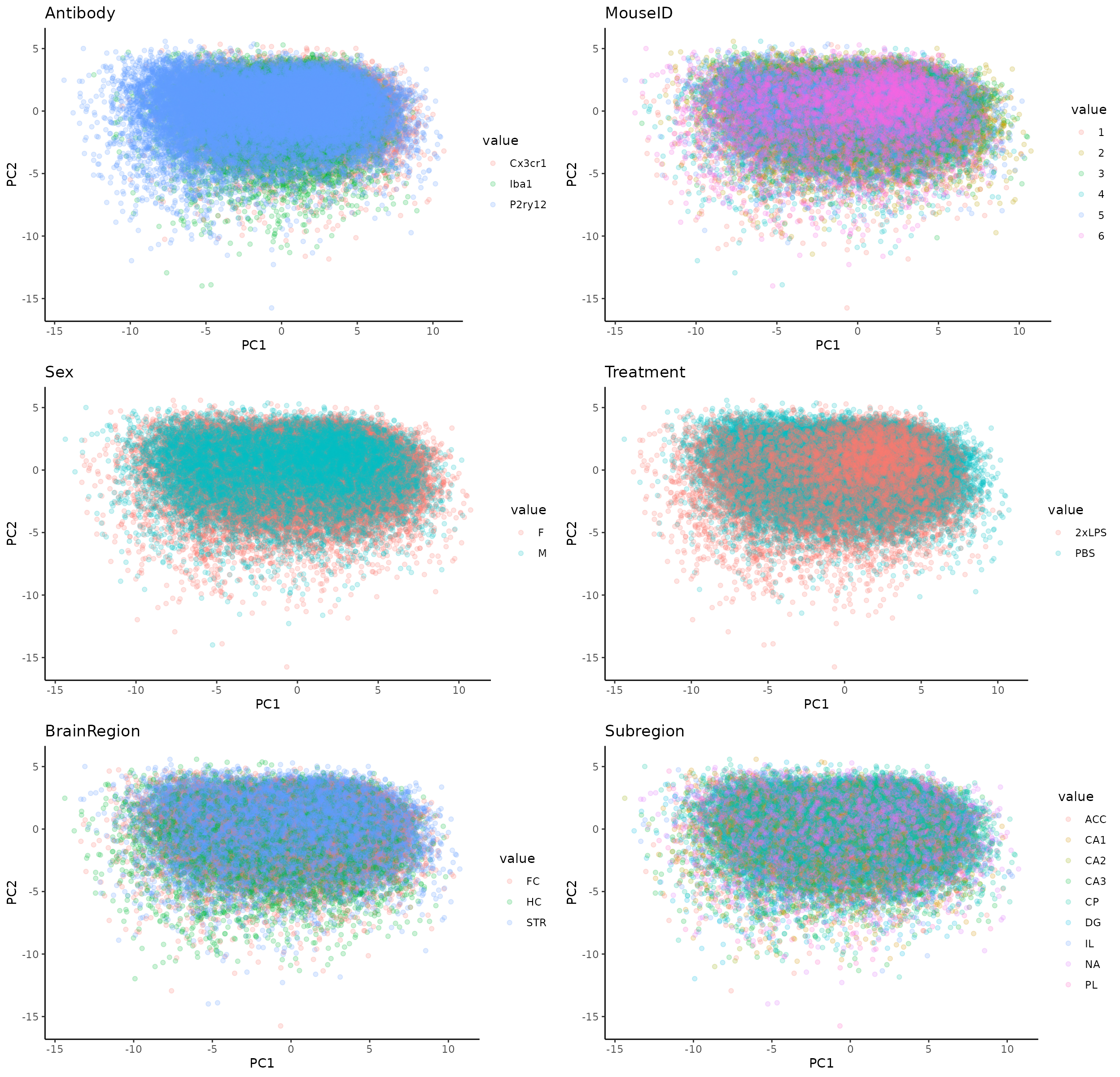
K-means clustering on PCs
After performing dimensionality reduction, we can use our PCs as input for downstream clustering methods. In this tutorial, we cluster our cells into morphological classes using k-means clustering, which partitions data points within a given dataset into defined numbers of clusters based on their proximity to the nearest cluster’s centroid. We provide an example at the end of the Github to depict a use case for fuzzy k-means clustering, a soft clustering approach and another option which allows for extended analyses such as characterization of the ‘most’ ameboid, hypertrophic, rod-like, or ramified cells or characterization of cells with more ambiguous identities that lie between these morphological states - see ‘Fuzzy K-means clustering’ section at the end of tutorial for more details about the method. Because our toolset is highly flexible, it can also be integrated with other clustering approaches such as hierarchical clustering or gaussian mixture models.
When running kmeans clustering, from the number of clusters (K) that you specify to create, the algorithm will randomly select K initial cluster centers. Each other data point’s euclidean distance will be calculated from these initial centers so that they are assigned as belonging to the cluster that they are closest to. The centroids for each of the clusters will be updated by calculating the new means of all the points assigned to each cluster. The process of randomly setting initial centers, assigning data points to the clusters, and updating the cluster centroids is iterated until the maximum number of iterations is reached.
Thus, 2 main dataset-specific parameters that you should specify and troubleshoot for your dataset are:
- iter.max, the maximum number of iterations allowed, and the number of times kmeans algorithm is run before results are returned. An iter.max between 10-20 is recommended
- nstart, how many random sets should be chosen. An nstart of atleast 25 initial configurations is recommended.
You can read more about kmeans clustering and optimizing these parameters at the following links:
Prepare data for clustering
## for k-means clustering: scale PCs 1-3, which together describe ~85% of variability
pca_data_scale <- transform_scale(pca_data, start=1, end=3) # scale pca data as input for k-means clustering
kmeans_input <- pca_data_scale[1:3]
Cluster optimization prior to running fuzzy k-means
# check for optimal number of clusters using wss and silhouette methods
sampling <- kmeans_input[sample(nrow(kmeans_input), 5000),] #sample 5000 random rows for cluster optimization

fviz_nbclust(sampling, kmeans, method = 'wss', nstart=25, iter.max=50) # 4 clusters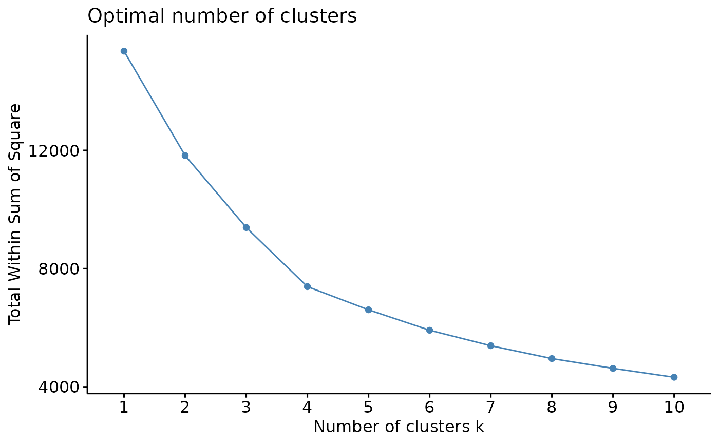
fviz_nbclust(sampling, kmeans, method = 'silhouette', nstart=25, iter.max=50) # 4 clusters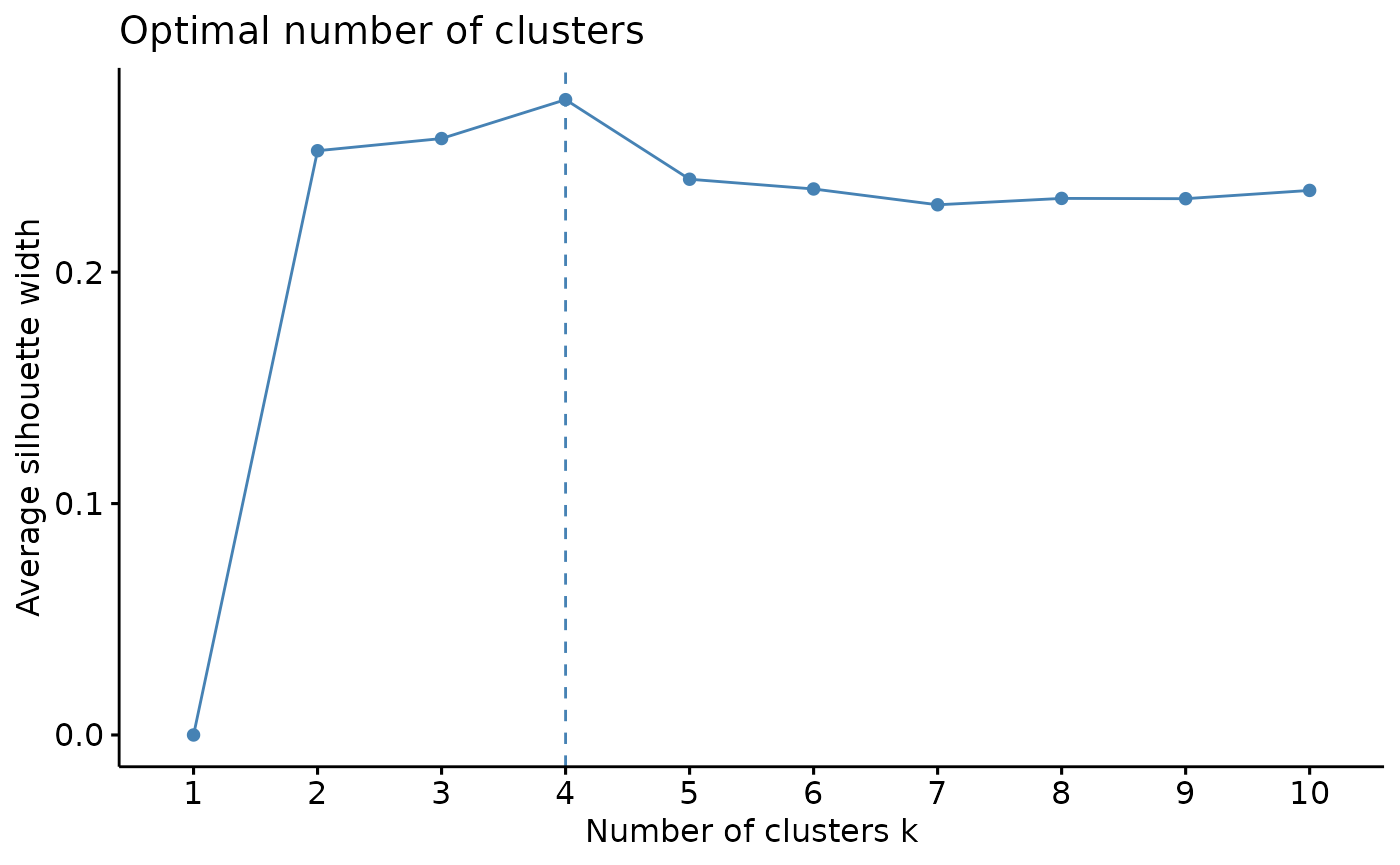
From using the wss and silhouette methods to check the optimal numbers of clusters for our dataset, it appears that our data would be optimally clustered using k=4. There are many more cluster optimization methods that you can try out to explore your data.
Next, we proceed with the actual clustering. You can cluster using fuzzy k-means or regular k-means at this step. After clustering, we will use some built-in functions within MicrogliaMorphologyR to assess how a parameter of k=4 influences how the clusters are defined by morphology features (and if they make sense according to what we know about microglia morphology). As this step may require some troubleshooting and updating of clustering parameters, you may need to run your k-means function multiple times. If you are planning to use fuzzy k-means, keep in mind that the soft clustering approach is more time-intensive and computationally expensive as it also calculates membership scores to each cluster for every single cell. It might help to use regular k-means as a first pass, verify that your clusters make sense using the functions that follow, and run your fuzzy k-means function using the final parameters that you determine to generate your final dataset for downstream analysis.
For the analysis proceeding, we are working with the regular k-means clustering output. We provide an example of a use case for fuzzy k-means clustering and further description of this approach at the end of the tutorial if you are interested.
Regular k-means (hard clustering)
# cluster and combine with original data
data_kmeans <- kmeans(kmeans_input, centers=4)

# Here, we are creating a new data frame that contains the first 2 PCs and original dataset, then renaming the data_kmeans$cluster column to simply say "Cluster". You can bind together as many of the PCs as you want. Binding the original, untransformed data is useful if you want to plot the raw values of any individual morphology measures downstream.
pca_kmeans <- cbind(pca_data[1:2], data_2xLPS, as.data.frame(data_kmeans$cluster)) %>%
  rename(Cluster=`data_kmeans$cluster`)
head(pca_kmeans,3)
#>           PC1       PC2 Antibody MouseID Sex Treatment BrainRegion Subregion
#> 1 -3.40837468 0.6764322   Cx3cr1       1   F     2xLPS          FC       ACC
#> 2 -3.97236479 0.6876435   Cx3cr1       1   F     2xLPS          FC       ACC
#> 3 -0.05205818 0.4984643   Cx3cr1       1   F     2xLPS          FC       ACC
#>            ID                                        UniqueID Foreground pixels
#> 1 00002-01053 Cx3cr1_Paper1_2Hit_1_F_2xLPS_FC_ACC_00002-01053              2535
#> 2 00009-01153 Cx3cr1_Paper1_2Hit_1_F_2xLPS_FC_ACC_00009-01153              2533
#> 3 00015-01224 Cx3cr1_Paper1_2Hit_1_F_2xLPS_FC_ACC_00015-01224              4996
#>   Density of foreground pixels in hull area
#> 1                                    0.6036
#> 2                                    0.6940
#> 3                                    0.6532
#>   Span ratio of hull (major/minor axis) Maximum span across hull Area Perimeter
#> 1                                1.2676                  90.5207 4200  263.8573
#> 2                                1.4896                  90.1388 3650  233.8153
#> 3                                1.4322                 128.9690 7648  350.8153
#>   Circularity Width of bounding rectangle Height of bounding rectangle
#> 1      0.7581                          81                           88
#> 2      0.8390                          67                           92
#> 3      0.7809                         107                          118
#>   Maximum radius from hull's center of mass
#> 1                                   50.6766
#> 2                                   49.8017
#> 3                                   66.6149
#>   Max/min radii from hull's center of mass
#> 1                                   1.7670
#> 2                                   1.9608
#> 3                                   1.8427
#>   Relative variation (CV) in radii from hull's center of mass Mean radius
#> 1                                                      0.1087     45.2033
#> 2                                                      0.1876     38.1056
#> 3                                                      0.1348     59.3454
#>   Diameter of bounding circle Maximum radius from circle's center of mass
#> 1                     98.5462                                     49.2731
#> 2                     90.1388                                     45.0694
#> 3                    131.2519                                     65.6259
#>   Max/min radii from circle's center of mass
#> 1                                     1.6904
#> 2                                     1.6125
#> 3                                     1.7132
#>   Relative variation (CV) in radii from circle's center of mass
#> 1                                                        0.1061
#> 2                                                        0.1704
#> 3                                                        0.1361
#>   Mean radius from circle's center of mass # of branches # of junctions
#> 1                                  44.9868            12              6
#> 2                                  37.4530            14              6
#> 3                                  59.4004            22             11
#>   # of end point voxels # of junction voxels # of slab voxels
#> 1                     6                   12              240
#> 2                     9                   14              208
#> 3                    10                   22              345
#>   Average branch length # of triple points # of quadruple points
#> 1                 8.729                  6                     0
#> 2                 6.722                  5                     1
#> 3                 7.173                 10                     1
#>   Maximum branch length Cluster
#> 1                29.236       4
#> 2                15.093       2
#> 3                21.261       3
Plot k-means clusters in PC space
plot <- clusterplots(pca_kmeans, "PC1", "PC2")
plot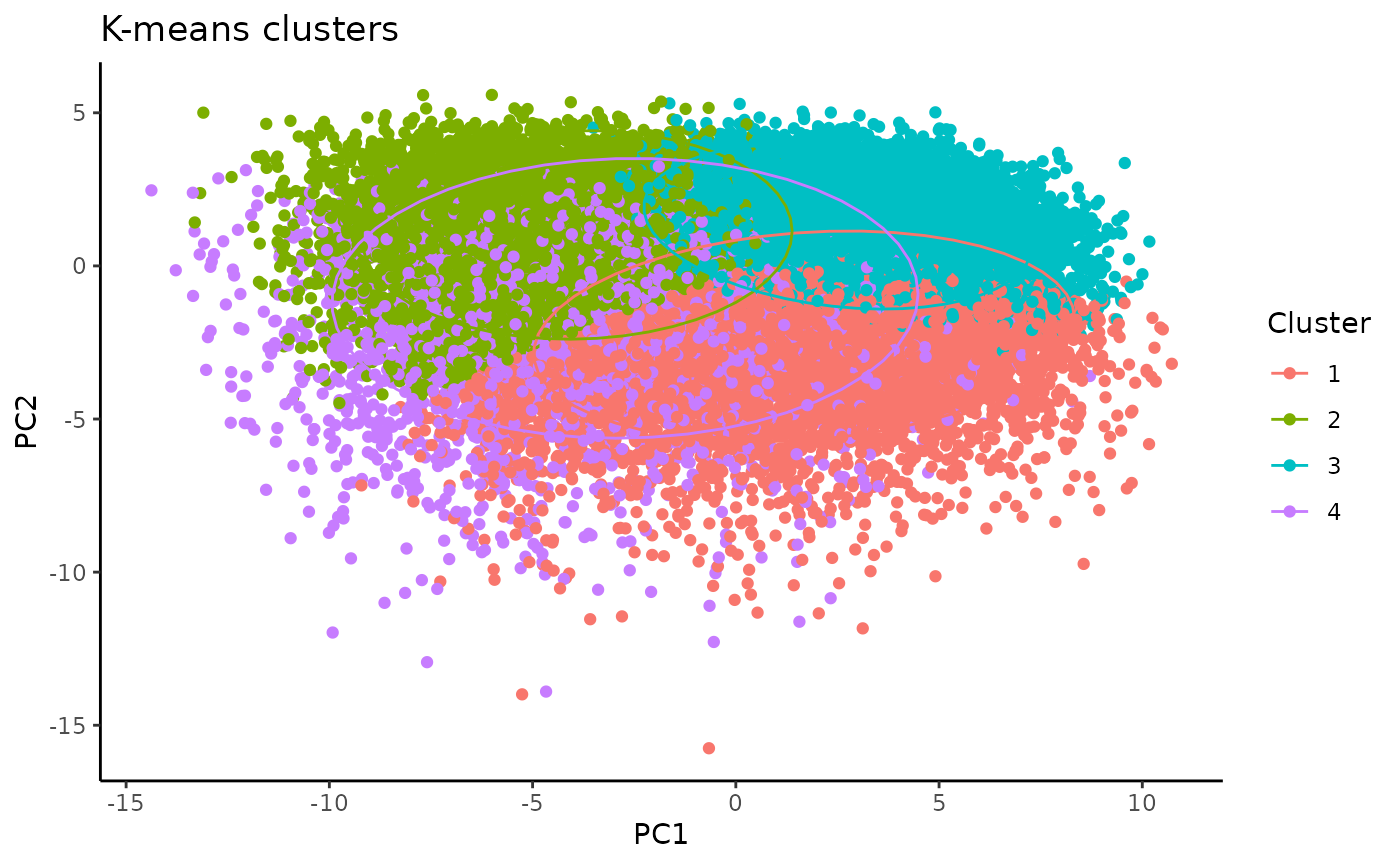
plot + scale_colour_viridis_d() # customizeable example: add color scheme of choice 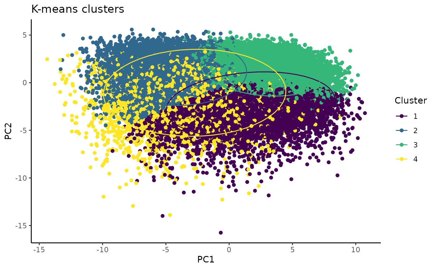
Cluster-specific measures on average for each morphology feature, relative to other clusters
clusterfeatures(pca_kmeans, featurestart=11, featureend=37)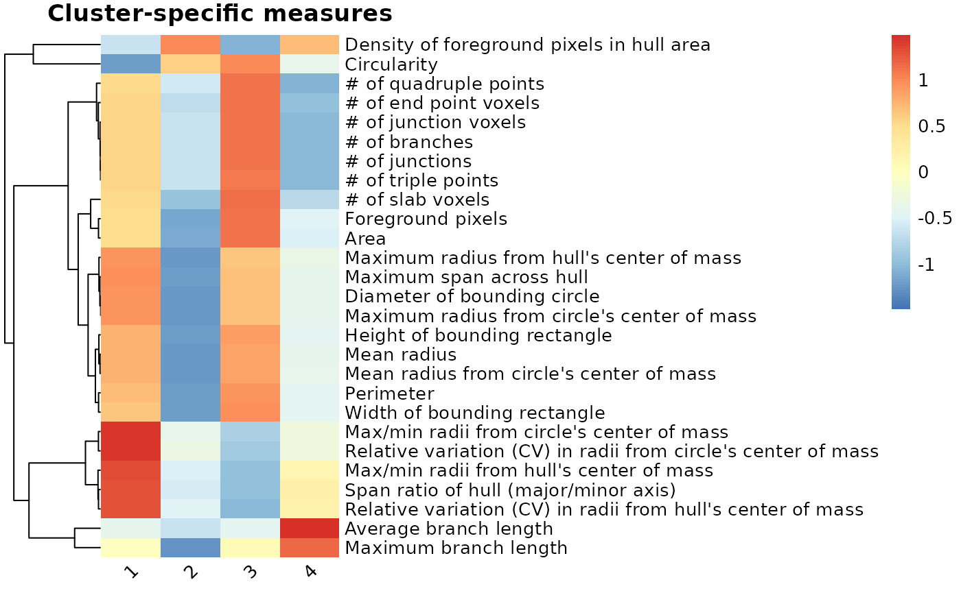
After comparing the individual features across clusters, we can characterize the clusters as follows:
- Cluster 1 = rod-like (greatest oblongness, lowest circularity)
- Cluster 2 = ameboid (lowest territory span, high circularity, smallest branch lengths)
- Cluster 3 = ramified (largest territory span and branching complexity)
- Cluster 4 = hypertrophic (average territory span, high branch thickness as explained by pixel density in hull)
ColorByCluster
Using the cluster classes assigned from our analyses using MicrogliaMorphologyR, we can color each cell in the original image by cluster using the MicrogliaMorphology ImageJ macro. In the following example, we are isolating out the Cluster assignments for each microglia in the Cx3cr1-stained ACC subregion image for Mouse 1. You can do this for all of the images you are interested in applying ColorByCluster to. This offers an additional method by which to visually assess and verify your suspected cluster identities before deeming them ramifed, hyper-ramified, rod-like, ameboid, or any other morphological form for downstream analysis and interpretation.
Make sure to filter for only the cells belonging to the image you want to run ColorByCluster on.
Formatting data for ColorByCluster input (Color coding in ImageJ)
# isolate out all the cells for your specific image of interest
colorbycluster <- pca_kmeans %>%
  filter(Antibody=="Cx3cr1",MouseID=="1", BrainRegion=="FC", Subregion=="ACC") %>% select(c(Cluster, ID))
head(colorbycluster)
#>   Cluster          ID
#> 1       4 00002-01053
#> 2       2 00009-01153
#> 3       3 00015-01224
#> 4       4 00016-01229
#> 5       4 00039-01394
#> 6       4 00044-01397
Save .csv file to feed into ColorByCluster function in MicrogliaMorphology ImageJ macro
write.csv(colorbycluster, "filepath/Cxc3cr_Mouse1_FC_ACC_data.csv")Cluster characterization
# calculate cluster percentages across variables of interest
cp <- clusterpercentage(pca_kmeans, "Cluster", MouseID, Antibody, Treatment, Sex, BrainRegion)
cp$Treatment <- factor(cp$Treatment, levels=c("PBS","2xLPS"))

# update cluster labels
cp <- cp %>% mutate(Cluster =
                      case_when(Cluster=="1" ~ "Rod-like",
                                Cluster=="2" ~ "Ameboid",
                                Cluster=="3" ~ "Ramified",
                                Cluster=="4" ~ "Hypertrophic"))

# Quick check of cluster proportions when considering experimental variables of interest
cp %>%
  filter(BrainRegion=="STR") %>% # in this example, we filter for our brain region of interest
  clusterpercentage_boxplots(Antibody, Treatment) # grouping variables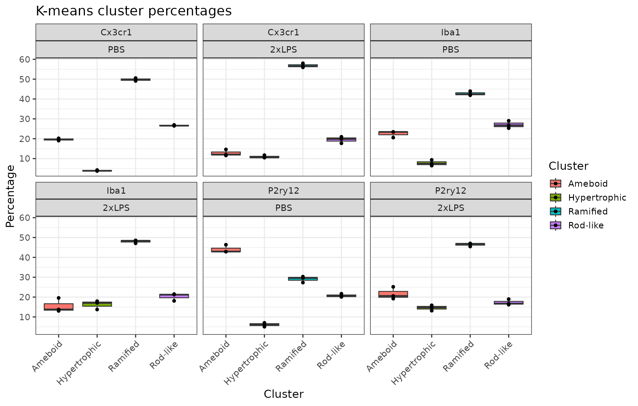
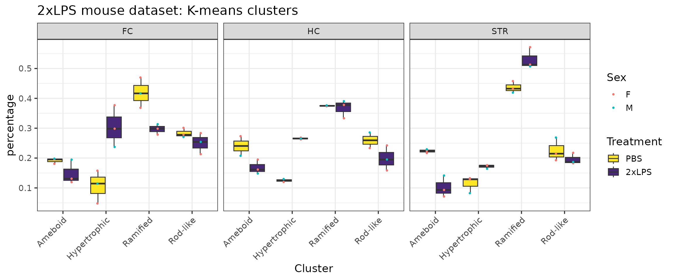
# example graph of data given variables of interest
cp %>%
  filter(Antibody=="Iba1") %>%
  ggplot(aes(x=Cluster, y=percentage, group=interaction(Cluster, Treatment))) +
  facet_wrap(~BrainRegion) +
  geom_boxplot(aes(group=interaction(Cluster, Treatment), fill=Treatment)) +
  scale_fill_manual(values=c("#fde725","#482878")) +
  geom_point(position=position_dodge(width=0.8), size=0.75, aes(group=interaction(Cluster,Treatment), color=Sex)) +
  ggtitle("2xLPS mouse dataset: K-means clusters") +
  labs(fill="Treatment") +
  theme_bw(base_size=14) +
  theme(axis.text.x=element_text(angle=45, vjust=1, hjust=1))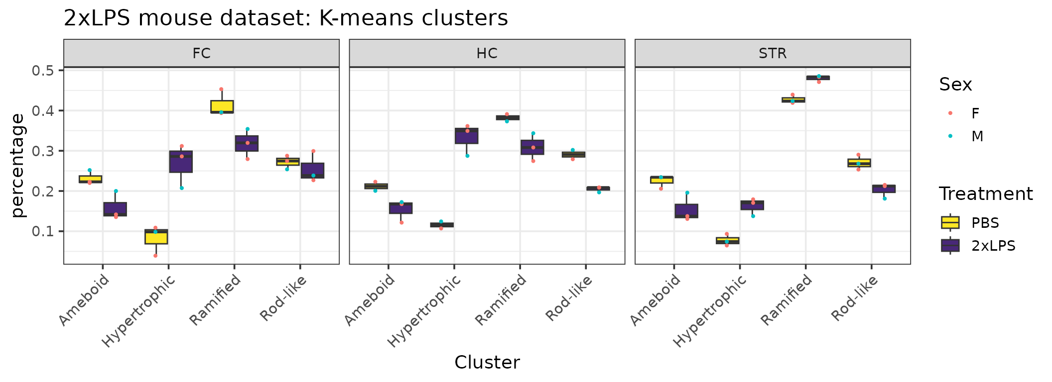
Statistical analysis
MicrogliaMorphologyR includes a few functions to run stats on cluster percentages as well as on individual morphology measures.
Cluster percentage changes at animal level, in response to experimental variables
e.g., Across clusters - How does cluster membership change with LPS?
The stats_cluster.animal function fits a generalized linear mixed
model on your dataset to a beta distribution, which is suitable for
values like percentages or probabilities that are constrained to a range
of 0-1, using the glmmTMB package. Part of the output
includes a check of the model fit using the DHARMa package,
which “uses a simulation-based approach to create readily interpretable
scaled (quantile) residuals for fitted (generalized) linear mixed
models.” The function creates two DHARMa plots, contained
in output[[4]]. You can read more about how to interpret model fit using
DHARMa by reading the package vignette.
In this example, we are fitting the generalized linear mixed model to our Iba1-stained dataset to model the percentage of cluster membership as a factor of Cluster identity, Treatment, and BrainRegion interactions with MouseID as a repeated measure since the outcome variable (cluster percentages) is represented multiple times per animal. In the first posthoc correction, we are correcting for multiple tests between treatments (PBS vs. 2xLPS) across Clusters and BrainRegions using the Bonferroni method - since there are 4 clusters and 3 brain regions, we should be correcting across 12 tests. In the second posthoc correction, we are correcting for multiple tests between treatments (PBS vs. 2xLPS) across Clusters using the Bonferroni method - since there are 4 clusters, we should be correcting across 4 tests.
# prepare percentages dataset for downstream analysis
stats.input <- cp
stats.input$MouseID <- factor(stats.input$MouseID)
stats.input$Cluster <- factor(stats.input$Cluster)
stats.input$Treatment <- factor(stats.input$Treatment)

# run stats analysis for changes in cluster percentages, at the animal level
# you can specify up to two posthoc comparisons (posthoc1 and posthoc2 arguments) - if you only have one set of posthocs to run, specify the same comparison twice for both arguments. you will just get the same results in output[[2]] and output[[3]].
stats.testing <- stats_cluster.animal(data = stats.input %>% filter(Antibody=="Iba1"),
                                      model = "percentage ~ Cluster*Treatment*BrainRegion + (1|MouseID)",
                                      posthoc1 = "~Treatment|Cluster|BrainRegion",
                                      posthoc2 = "~Treatment|Cluster", adjust = "bonferroni")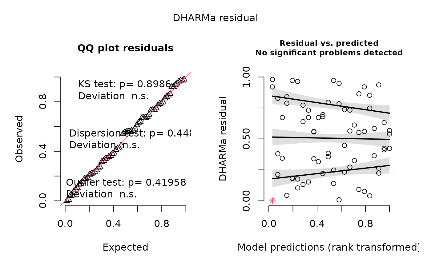
#> NOTE: Results may be misleading due to involvement in interactions
#> Formula:
#> percentage ~ Cluster * Treatment * BrainRegion + (1 | MouseID)
#> Data: data
#>       AIC       BIC    logLik  df.resid
#> -264.2217 -206.5145  158.1109        42
#> Random-effects (co)variances:
#>
#> Conditional model:
#>  Groups  Name        Std.Dev.
#>  MouseID (Intercept) 2.66e-06
#>
#> Number of obs: 68 / Conditional model: MouseID, 6
#>
#> Dispersion parameter for beta family ():  296
#>
#> Fixed Effects:
#>
#> Conditional model:
#>                      (Intercept)                          Cluster1
#>                        -1.190535                         -0.280517
#>                         Cluster2                          Cluster3
#>                        -0.530336                          0.729137
#>                       Treatment1                      BrainRegion1
#>                        -0.034300                         -0.001085
#>                     BrainRegion2               Cluster1:Treatment1
#>                         0.032280                          0.258393
#>              Cluster2:Treatment1               Cluster3:Treatment1
#>                        -0.571027                          0.123271
#>            Cluster1:BrainRegion1             Cluster2:BrainRegion1
#>                         0.038133                         -0.026514
#>            Cluster3:BrainRegion1             Cluster1:BrainRegion2
#>                        -0.093337                         -0.070106
#>            Cluster2:BrainRegion2             Cluster3:BrainRegion2
#>                         0.327990                         -0.213648
#>          Treatment1:BrainRegion1           Treatment1:BrainRegion2
#>                        -0.026359                          0.016676
#> Cluster1:Treatment1:BrainRegion1  Cluster2:Treatment1:BrainRegion1
#>                         0.040356                         -0.105077
#> Cluster3:Treatment1:BrainRegion1  Cluster1:Treatment1:BrainRegion2
#>                         0.146770                         -0.041974
#> Cluster2:Treatment1:BrainRegion2  Cluster3:Treatment1:BrainRegion2
#>                        -0.074843                          0.057942

stats.testing[[1]] # anova
#> Analysis of Deviance Table (Type II Wald chisquare tests)
#>
#> Response: percentage
#>                                  Chisq Df Pr(>Chisq)
#> Cluster                       632.4490  3  < 2.2e-16 ***
#> Treatment                       1.2604  1     0.2616
#> BrainRegion                     0.2084  2     0.9010
#> Cluster:Treatment             271.0010  3  < 2.2e-16 ***
#> Cluster:BrainRegion           120.9206  6  < 2.2e-16 ***
#> Treatment:BrainRegion           2.0685  2     0.3555
#> Cluster:Treatment:BrainRegion  38.4144  6  9.321e-07 ***
#> ---
#> Signif. codes:  0 '***' 0.001 '**' 0.01 '*' 0.05 '.' 0.1 ' ' 1
stats.testing[[2]] # posthoc 1
#>  contrast    Cluster      BrainRegion   estimate         SE  df z.ratio p.value
#>  PBS - 2xLPS Ameboid      FC           0.4761807 0.12097420 Inf   3.936  0.0010
#>  PBS - 2xLPS Hypertrophic FC          -1.4735259 0.14575411 Inf -10.110  <.0001
#>  PBS - 2xLPS Ramified     FC           0.4187653 0.09890622 Inf   4.234  0.0003
#>  PBS - 2xLPS Rod-like     FC           0.0933095 0.10739882 Inf   0.869  1.0000
#>  PBS - 2xLPS Ameboid      HC           0.3975891 0.13631860 Inf   2.917  0.0425
#>  PBS - 2xLPS Hypertrophic HC          -1.3269892 0.14559100 Inf  -9.114  <.0001
#>  PBS - 2xLPS Ramified     HC           0.3271791 0.11116899 Inf   2.943  0.0390
#>  PBS - 2xLPS Rod-like     HC           0.4612293 0.12234620 Inf   3.770  0.0020
#>  PBS - 2xLPS Ameboid      STR          0.4707880 0.12231265 Inf   3.849  0.0014
#>  PBS - 2xLPS Hypertrophic STR         -0.8314493 0.15327901 Inf  -5.424  <.0001
#>  PBS - 2xLPS Ramified     STR         -0.2121166 0.09521815 Inf  -2.228  0.3108
#>  PBS - 2xLPS Rod-like     STR          0.3758423 0.11203994 Inf   3.355  0.0095
#>  Significant
#>  significant
#>  significant
#>  significant
#>  ns
#>  significant
#>  significant
#>  significant
#>  significant
#>  significant
#>  significant
#>  ns
#>  significant
#>
#> Results are given on the log odds ratio (not the response) scale.
#> P value adjustment: bonferroni method for 12 tests
stats.testing[[3]] # posthoc 2
#>  contrast    Cluster        estimate         SE  df z.ratio p.value Significant
#>  PBS - 2xLPS Ameboid       0.4481859 0.07316650 Inf   6.126  <.0001 significant
#>  PBS - 2xLPS Hypertrophic -1.2106548 0.08561029 Inf -14.141  <.0001 significant
#>  PBS - 2xLPS Ramified      0.1779426 0.05888547 Inf   3.022  0.0100 significant
#>  PBS - 2xLPS Rod-like      0.3101270 0.06587576 Inf   4.708  <.0001 significant
#>
#> Results are averaged over the levels of: BrainRegion
#> Results are given on the log odds ratio (not the response) scale.
#> P value adjustment: bonferroni method for 4 tests
stats.testing[[4]] # DHARMa model check
stats.testing[[5]] # summary of model
#> Formula:
#> percentage ~ Cluster * Treatment * BrainRegion + (1 | MouseID)
#> Data: data
#>       AIC       BIC    logLik  df.resid
#> -264.2217 -206.5145  158.1109        42
#> Random-effects (co)variances:
#>
#> Conditional model:
#>  Groups  Name        Std.Dev.
#>  MouseID (Intercept) 2.66e-06
#>
#> Number of obs: 68 / Conditional model: MouseID, 6
#>
#> Dispersion parameter for beta family ():  296
#>
#> Fixed Effects:
#>
#> Conditional model:
#>                      (Intercept)                          Cluster1
#>                        -1.190535                         -0.280517
#>                         Cluster2                          Cluster3
#>                        -0.530336                          0.729137
#>                       Treatment1                      BrainRegion1
#>                        -0.034300                         -0.001085
#>                     BrainRegion2               Cluster1:Treatment1
#>                         0.032280                          0.258393
#>              Cluster2:Treatment1               Cluster3:Treatment1
#>                        -0.571027                          0.123271
#>            Cluster1:BrainRegion1             Cluster2:BrainRegion1
#>                         0.038133                         -0.026514
#>            Cluster3:BrainRegion1             Cluster1:BrainRegion2
#>                        -0.093337                         -0.070106
#>            Cluster2:BrainRegion2             Cluster3:BrainRegion2
#>                         0.327990                         -0.213648
#>          Treatment1:BrainRegion1           Treatment1:BrainRegion2
#>                        -0.026359                          0.016676
#> Cluster1:Treatment1:BrainRegion1  Cluster2:Treatment1:BrainRegion1
#>                         0.040356                         -0.105077
#> Cluster3:Treatment1:BrainRegion1  Cluster1:Treatment1:BrainRegion2
#>                         0.146770                         -0.041974
#> Cluster2:Treatment1:BrainRegion2  Cluster3:Treatment1:BrainRegion2
#>                        -0.074843                          0.057942
Individual morphology measures, at the animal level (averaged across cells for each animal)
e.g., How does each individual morphology measure change with LPS treatment?
The stats_morphologymeasures.animal function fits a linear model
using the lm function for each morphology measure
individually within your dataset.
In this example, we are fitting the linear model to our Iba1-stained dataset to model the values of each morphology measure as a factor of Treatment and BrainRegion interactions. In the first posthoc correction, we are correcting for multiple comparisons between treatments (PBS vs. 2xLPS) across BrainRegions using the Bonferroni method - since there are 3 brain regions, we should be correcting across 3 tests for each morphology measure. In the second posthoc correction, we are correcting for multiple comparisons between every individual interaction of treatment (PBS or 2xLPS) and brain region (FC, HC, STR) against the others (e.g., 2xLPS FC vs. PBS STR) and should be correcting across 15 tests for each morphology measure. In the second example, we are testing all possible comparisons given the experimental variables in our model, and are thus considering many tests that aren’t biologically relevant or useful in our experiment.
# prepare data for downstream analysis
data <- data_2xLPS %>%
  group_by(MouseID, Sex, Treatment, BrainRegion, Antibody) %>%
  summarise(across("Foreground pixels":"Maximum branch length", ~mean(.x))) %>%
  gather(Measure, Value, "Foreground pixels":"Maximum branch length")
#> `summarise()` has grouped output by 'MouseID', 'Sex', 'Treatment',
#> 'BrainRegion'. You can override using the `.groups` argument.

# filter out data you want to run stats on and make sure to make any variables included in model into factors
stats.input <- data
stats.input$Treatment <- factor(stats.input$Treatment)

# run stats analysis for changes in individual morphology measures
# you can specify up to two posthoc comparisons (posthoc1 and posthoc2 arguments) - if you only have one set of posthocs to run, specify the same comparison twice for both arguments. you will just get the same results in output[[2]] and output[[3]].
stats.testing <- stats_morphologymeasures.animal(data = stats.input %>% filter(Antibody=="Iba1"),
                                                 model = "Value ~ Treatment*BrainRegion", type="lm",
                                                 posthoc1 = "~Treatment|BrainRegion",
                                                 posthoc2 = "~Treatment*BrainRegion", adjust = "bonferroni")
#> [1] "Foreground pixels"
#> [1] "Density of foreground pixels in hull area"
#> [1] "Span ratio of hull (major/minor axis)"
#> [1] "Maximum span across hull"
#> [1] "Area"
#> [1] "Perimeter"
#> [1] "Circularity"
#> [1] "Width of bounding rectangle"
#> [1] "Height of bounding rectangle"
#> [1] "Maximum radius from hull's center of mass"
#> [1] "Max/min radii from hull's center of mass"
#> [1] "Relative variation (CV) in radii from hull's center of mass"
#> [1] "Mean radius"
#> [1] "Diameter of bounding circle"
#> [1] "Maximum radius from circle's center of mass"
#> [1] "Max/min radii from circle's center of mass"
#> [1] "Relative variation (CV) in radii from circle's center of mass"
#> [1] "Mean radius from circle's center of mass"
#> [1] "# of branches"
#> [1] "# of junctions"
#> [1] "# of end point voxels"
#> [1] "# of junction voxels"
#> [1] "# of slab voxels"
#> [1] "Average branch length"
#> [1] "# of triple points"
#> [1] "# of quadruple points"
#> [1] "Maximum branch length"

# anova
stats.testing[[1]] %>% head(8)
#>                              Sum Sq Df   F value       Pr(>F)
#> Treatment              6.875349e+05  1 65.060279 6.040851e-06
#> BrainRegion            6.273589e+04  2  2.968296 9.313579e-02
#> Treatment:BrainRegion  6.182606e+04  2  2.925248 9.578334e-02
#> Residuals              1.162443e+05 11        NA           NA
#> Treatment1             2.318244e-02  1 61.707786 7.765694e-06
#> BrainRegion1           5.230256e-03  2  6.961034 1.112878e-02
#> Treatment:BrainRegion1 1.396941e-03  2  1.859211 2.015685e-01
#> Residuals1             4.132491e-03 11        NA           NA
#>                                                          measure Significant
#> Treatment                                      Foreground pixels significant
#> BrainRegion                                    Foreground pixels          ns
#> Treatment:BrainRegion                          Foreground pixels          ns
#> Residuals                                      Foreground pixels        <NA>
#> Treatment1             Density of foreground pixels in hull area significant
#> BrainRegion1           Density of foreground pixels in hull area significant
#> Treatment:BrainRegion1 Density of foreground pixels in hull area          ns
#> Residuals1             Density of foreground pixels in hull area        <NA>
# posthoc 1
stats.testing[[2]] %>% head(6)
#>      contrast BrainRegion     estimate          SE df  t.ratio      p.value
#> 1 2xLPS - PBS          FC 244.19621196 83.93513466 11 2.909344 0.0426170253
#> 2 2xLPS - PBS          HC 464.89704224 93.84233340 11 4.954023 0.0012985925
#> 3 2xLPS - PBS         STR 516.75796274 83.93513466 11 6.156635 0.0002142012
#> 4 2xLPS - PBS          FC   0.07300851  0.01582574 11 4.613277 0.0022456005
#> 5 2xLPS - PBS          HC   0.10040427  0.01769371 11 5.674573 0.0004304675
#> 6 2xLPS - PBS         STR   0.05469185  0.01582574 11 3.455880 0.0161161442
#>                                     measure Significant
#> 1                         Foreground pixels significant
#> 2                         Foreground pixels significant
#> 3                         Foreground pixels significant
#> 4 Density of foreground pixels in hull area significant
#> 5 Density of foreground pixels in hull area significant
#> 6 Density of foreground pixels in hull area significant
# posthoc 2
stats.testing[[3]] %>% head(6)
#>               contrast   estimate       SE df    t.ratio     p.value
#> 1    2xLPS FC - PBS FC  244.19621 83.93513 11  2.9093444 0.213085126
#> 2  2xLPS FC - 2xLPS HC   37.26016 83.93513 11  0.4439162 1.000000000
#> 3    2xLPS FC - PBS HC  502.15721 93.84233 11  5.3510733 0.003501430
#> 4 2xLPS FC - 2xLPS STR  -25.72618 83.93513 11 -0.3065007 1.000000000
#> 5   2xLPS FC - PBS STR  491.03178 83.93513 11  5.8501340 0.001663025
#> 6    PBS FC - 2xLPS HC -206.93605 83.93513 11 -2.4654282 0.470625546
#>             measure Significant
#> 1 Foreground pixels          ns
#> 2 Foreground pixels          ns
#> 3 Foreground pixels significant
#> 4 Foreground pixels          ns
#> 5 Foreground pixels significant
#> 6 Foreground pixels          ns
# qqplots to check normality assumptions
do.call("grid.arrange", c(stats.testing[[4]], ncol=4))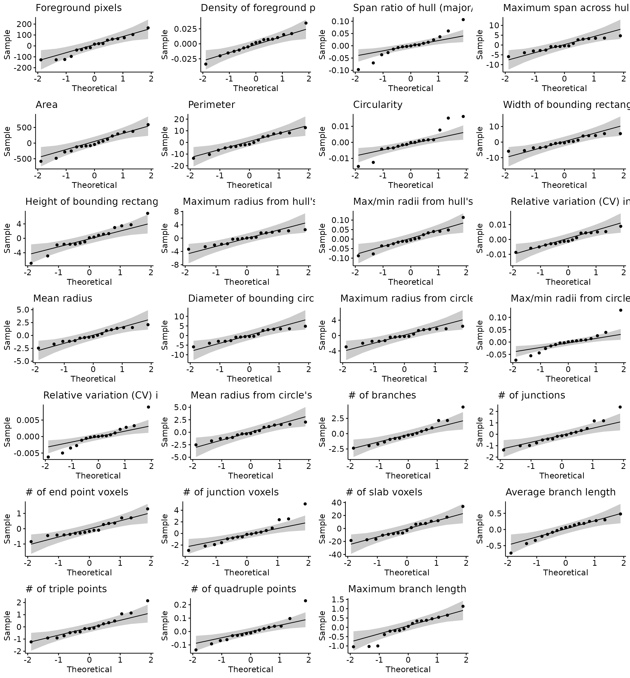
# shapiro test
stats.testing[[5]] %>% head(6)
#>           variable statistic   p.value pass
#> 1 residuals(model) 0.9541450 0.5252634 pass
#> 2 residuals(model) 0.9874225 0.9958905 pass
#> 3 residuals(model) 0.9518543 0.4865020 pass
#> 4 residuals(model) 0.9481459 0.4278652 pass
#> 5 residuals(model) 0.9832680 0.9809502 pass
#> 6 residuals(model) 0.9770036 0.9250129 pass
#>                                     measure
#> 1                         Foreground pixels
#> 2 Density of foreground pixels in hull area
#> 3     Span ratio of hull (major/minor axis)
#> 4                  Maximum span across hull
#> 5                                      Area
#> 6                                 Perimeter
If you are not interested in running stats for all 27 morphology
measures, you can also filter for those that you are interested in (or
filter out those that you’re not interested in) prior to running the
stats_morphologymeasures.animal function. In this example,
we filter out 4 morphology measures so that we only run this function on
the other 23 measures.
# run stats analysis for changes in individual morphology measures
# you can specify up to two posthoc comparisons (posthoc1 and posthoc2 arguments) - if you only have one set of posthocs to run, specify the same comparison twice for both arguments. you will just get the same results in output[[2]] and output[[3]].

stats.input_filtered <- stats.input %>%
  filter(Antibody=="Iba1") %>%
  filter(!Measure %in% c("Foreground pixels",
                         "Average branch length",
                         "# of quadruple points",
                         "Height of bounding rectangle"))
stats.testing <- stats_morphologymeasures.animal(data = stats.input_filtered,
                                                 model = "Value ~ Treatment*BrainRegion", type = "lm",
                                                 posthoc1 = "~Treatment|BrainRegion",
                                                 posthoc2 = "~Treatment*BrainRegion", adjust ="bonferroni")
#> [1] "Density of foreground pixels in hull area"
#> [1] "Span ratio of hull (major/minor axis)"
#> [1] "Maximum span across hull"
#> [1] "Area"
#> [1] "Perimeter"
#> [1] "Circularity"
#> [1] "Width of bounding rectangle"
#> [1] "Maximum radius from hull's center of mass"
#> [1] "Max/min radii from hull's center of mass"
#> [1] "Relative variation (CV) in radii from hull's center of mass"
#> [1] "Mean radius"
#> [1] "Diameter of bounding circle"
#> [1] "Maximum radius from circle's center of mass"
#> [1] "Max/min radii from circle's center of mass"
#> [1] "Relative variation (CV) in radii from circle's center of mass"
#> [1] "Mean radius from circle's center of mass"
#> [1] "# of branches"
#> [1] "# of junctions"
#> [1] "# of end point voxels"
#> [1] "# of junction voxels"
#> [1] "# of slab voxels"
#> [1] "# of triple points"
#> [1] "Maximum branch length"

# anova
stats.testing[[1]] %>% head(8)
#>                              Sum Sq Df    F value       Pr(>F)
#> Treatment              0.0231824401  1 61.7077864 7.765694e-06
#> BrainRegion            0.0052302556  2  6.9610338 1.112878e-02
#> Treatment:BrainRegion  0.0013969407  2  1.8592115 2.015685e-01
#> Residuals              0.0041324905 11         NA           NA
#> Treatment1             0.0008300607  1  0.2688058 6.144032e-01
#> BrainRegion1           0.0437404668  2  7.0824290 1.055091e-02
#> Treatment:BrainRegion1 0.0223637009  2  3.6211164 6.190572e-02
#> Residuals1             0.0339675228 11         NA           NA
#>                                                          measure Significant
#> Treatment              Density of foreground pixels in hull area significant
#> BrainRegion            Density of foreground pixels in hull area significant
#> Treatment:BrainRegion  Density of foreground pixels in hull area          ns
#> Residuals              Density of foreground pixels in hull area        <NA>
#> Treatment1                 Span ratio of hull (major/minor axis)          ns
#> BrainRegion1               Span ratio of hull (major/minor axis) significant
#> Treatment:BrainRegion1     Span ratio of hull (major/minor axis)          ns
#> Residuals1                 Span ratio of hull (major/minor axis)        <NA>
# posthoc 1
stats.testing[[2]] %>% head(6)
#>      contrast BrainRegion    estimate         SE df    t.ratio      p.value
#> 1 2xLPS - PBS          FC  0.07300851 0.01582574 11  4.6132766 0.0022456005
#> 2 2xLPS - PBS          HC  0.10040427 0.01769371 11  5.6745733 0.0004304675
#> 3 2xLPS - PBS         STR  0.05469185 0.01582574 11  3.4558799 0.0161161442
#> 4 2xLPS - PBS          FC  0.09192749 0.04537221 11  2.0260747 0.2031182136
#> 5 2xLPS - PBS          HC  0.03246885 0.05072768 11  0.6400618 1.0000000000
#> 6 2xLPS - PBS         STR -0.07853956 0.04537221 11 -1.7310057 0.3340946601
#>                                     measure Significant
#> 1 Density of foreground pixels in hull area significant
#> 2 Density of foreground pixels in hull area significant
#> 3 Density of foreground pixels in hull area significant
#> 4     Span ratio of hull (major/minor axis)          ns
#> 5     Span ratio of hull (major/minor axis)          ns
#> 6     Span ratio of hull (major/minor axis)          ns
# posthoc 2
stats.testing[[3]] %>% head(6)
#>               contrast     estimate         SE df   t.ratio      p.value
#> 1    2xLPS FC - PBS FC  0.073008506 0.01582574 11  4.613277 0.0112280026
#> 2  2xLPS FC - 2xLPS HC -0.004762487 0.01582574 11 -0.300933 1.0000000000
#> 3    2xLPS FC - PBS HC  0.095641782 0.01769371 11  5.405411 0.0032232825
#> 4 2xLPS FC - 2xLPS STR  0.048370714 0.01582574 11  3.056459 0.1638120520
#> 5   2xLPS FC - PBS STR  0.103062562 0.01582574 11  6.512339 0.0006530396
#> 6    PBS FC - 2xLPS HC -0.077770993 0.01582574 11 -4.914210 0.0069162488
#>                                     measure Significant
#> 1 Density of foreground pixels in hull area significant
#> 2 Density of foreground pixels in hull area          ns
#> 3 Density of foreground pixels in hull area significant
#> 4 Density of foreground pixels in hull area          ns
#> 5 Density of foreground pixels in hull area significant
#> 6 Density of foreground pixels in hull area significant
# qqplots to check normality assumptions
do.call("grid.arrange", c(stats.testing[[4]], ncol=4))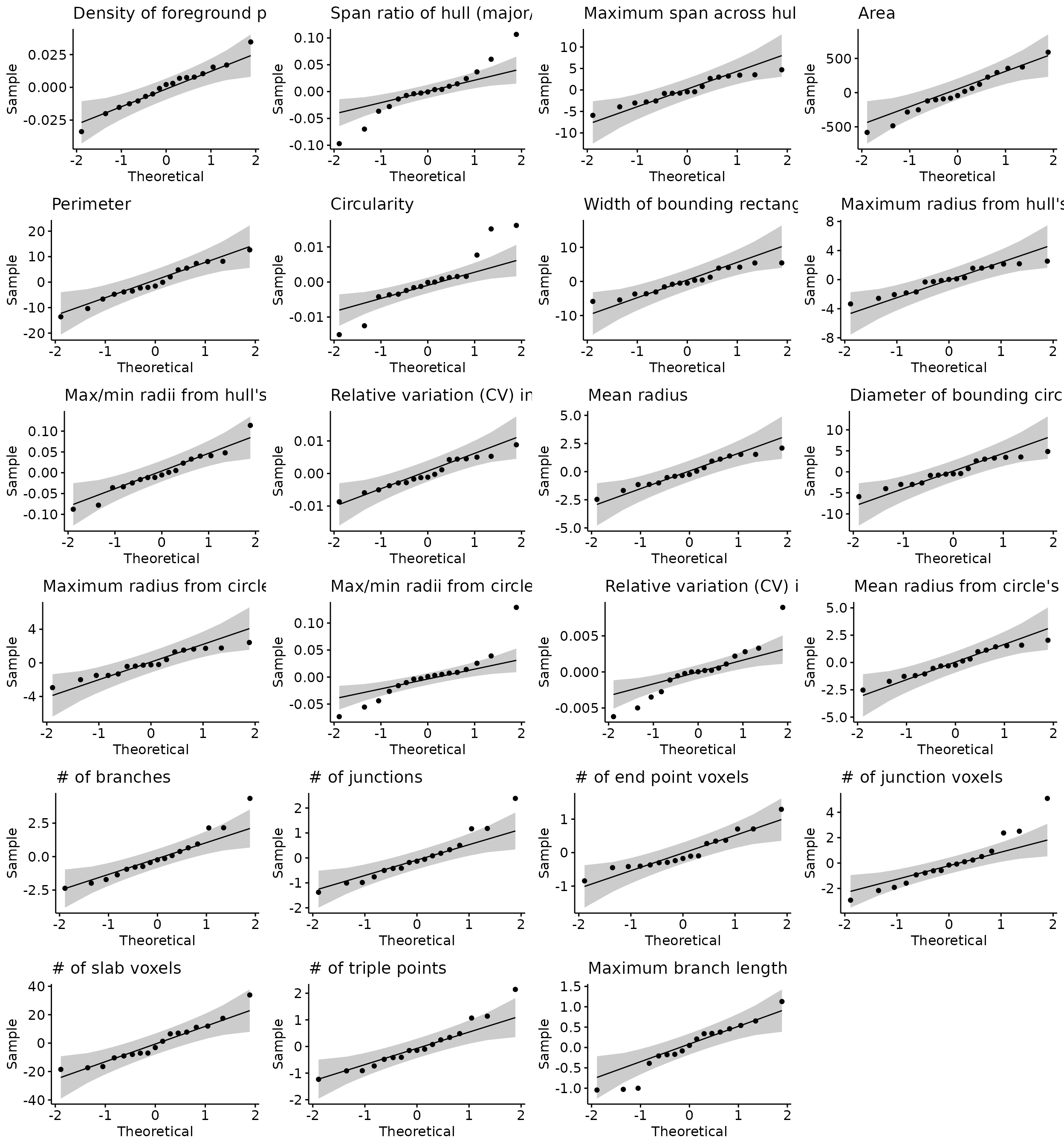
# shapiro test
stats.testing[[5]] %>% head(6)
#>           variable statistic    p.value pass
#> 1 residuals(model) 0.9874225 0.99589048 pass
#> 2 residuals(model) 0.9518543 0.48650203 pass
#> 3 residuals(model) 0.9481459 0.42786519 pass
#> 4 residuals(model) 0.9832680 0.98095021 pass
#> 5 residuals(model) 0.9770036 0.92501287 pass
#> 6 residuals(model) 0.9079043 0.09221502 pass
#>                                     measure
#> 1 Density of foreground pixels in hull area
#> 2     Span ratio of hull (major/minor axis)
#> 3                  Maximum span across hull
#> 4                                      Area
#> 5                                 Perimeter
#> 6                               Circularity
If you find that any individual morphology measures violate
assumptions of normality after checking the qqplots contained in
stats.input[[4]], you can filter your data for those measures, transform
your data in the suitable manner (i.e., using MicrogliaMorphologyR
functions like transform_minmax or
transform_scale or other data transformations), and rerun
the stats for those morphology features using the code above.
Fuzzy K-means Clustering
To cluster your cells into morphological classes, you can use regular k-means or fuzzy k-means clustering. We provide an example of using fuzzy k-means, a ‘soft’ clustering method that is similar in concept and algorithm to k-means clustering, which partitions data points within a given dataset into defined numbers of clusters based on their proximity to the nearest cluster’s centroid. In fuzzy k-means, data points are not exclusively assigned to just one cluster, but rather given membership scores to all clusters. This allows for additional characterization of high-scoring cells within each cluster (i.e., quintessential ‘rod-like’, ‘ameboid’, ‘hypertrophic’, or ‘ramified’ cells), cells with more ambiguous identities (e.g., a cell that is 5% rod-like, 5% ameboid, 45% hypertrophic, and 45% ramified), and other cases that the user might be interested in which might be informative for their specific dataset. Fuzzy k-means also assigns a final hard cluster assignment based on the class with the highest membership score, which can be used as input for analysis as well. Here, we include an example of one use case of the membership scores provided by fuzzy k-means.
Example of additional analyses possible with fuzzy k-means (soft clustering) membership scores
Here, we will use a fuzzy k-means dataset that comes pre-loaded with
the package for demonstration purposes, as running the actual fuzzy
clustering step using the fcm function in the
ppclust package
is time-intensive and computationally-expensive.
Load in example dataset:
data_fuzzykmeans <- MicrogliaMorphologyR::data_2xLPS_mouse_fuzzykmeans
colnames(data_fuzzykmeans)
#>  [1] "Antibody"
#>  [2] "MouseID"
#>  [3] "Sex"
#>  [4] "Treatment"
#>  [5] "BrainRegion"
#>  [6] "Subregion"
#>  [7] "ID"
#>  [8] "UniqueID"
#>  [9] "Foreground pixels"
#> [10] "Density of foreground pixels in hull area"
#> [11] "Span ratio of hull (major/minor axis)"
#> [12] "Maximum span across hull"
#> [13] "Area"
#> [14] "Perimeter"
#> [15] "Circularity"
#> [16] "Width of bounding rectangle"
#> [17] "Height of bounding rectangle"
#> [18] "Maximum radius from hull's center of mass"
#> [19] "Max/min radii from hull's center of mass"
#> [20] "Relative variation (CV) in radii from hull's center of mass"
#> [21] "Mean radius"
#> [22] "Diameter of bounding circle"
#> [23] "Maximum radius from circle's center of mass"
#> [24] "Max/min radii from circle's center of mass"
#> [25] "Relative variation (CV) in radii from circle's center of mass"
#> [26] "Mean radius from circle's center of mass"
#> [27] "# of branches"
#> [28] "# of junctions"
#> [29] "# of end point voxels"
#> [30] "# of junction voxels"
#> [31] "# of slab voxels"
#> [32] "Average branch length"
#> [33] "# of triple points"
#> [34] "# of quadruple points"
#> [35] "Maximum branch length"
#> [36] "PC1"
#> [37] "PC2"
#> [38] "PC3"
#> [39] "Cluster 1"
#> [40] "Cluster 2"
#> [41] "Cluster 3"
#> [42] "Cluster 4"
#> [43] "Cluster"

# check cluster features to determine cluster labels
clusterfeatures(data_fuzzykmeans, featurestart=9, featureend=35)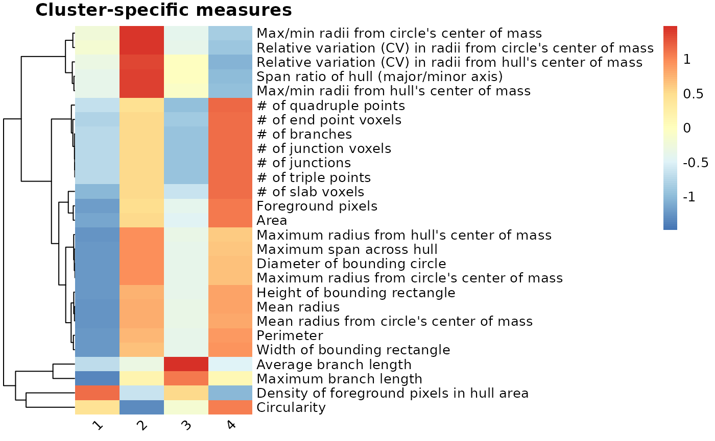
# update cluster labels
data_fuzzykmeans <- data_fuzzykmeans %>% mutate(Cluster =
                      case_when(Cluster=="1" ~ "Ameboid",
                                Cluster=="2" ~ "Rod-like",
                                Cluster=="3" ~ "Hypertrophic",
                                Cluster=="4" ~ "Ramified"))
Example: Characterization of just the high-scoring cells within each cluster (i.e., quintessential ‘rod-like’, ‘ameboid’, ‘hypertrophic’, or ‘ramified’ cells)
nrow(data_fuzzykmeans) # number of cells prior to filtering
#> [1] 43332

# filter for high-scoring cells, defined as >70% membership score in one of the clusters
data <- data_fuzzykmeans %>%
  filter(`Cluster 1` > 0.70|
         `Cluster 2` > 0.70|
         `Cluster 3` > 0.70|
         `Cluster 4` > 0.70)

nrow(data) # number of cells after filtering for just the high-scoring cells
#> [1] 7525

# calculate cluster percentages across variables of interest
cp <- clusterpercentage(data, "Cluster", MouseID, Antibody, Treatment, Sex, BrainRegion)
cp$Treatment <- factor(cp$Treatment, levels=c("PBS","2xLPS"))

# example graph of data given variables of interest
cp %>%
  filter(Antibody=="Iba1") %>%
  ggplot(aes(x=Cluster, y=percentage, group=interaction(Cluster, Treatment))) +
  facet_wrap(~BrainRegion) +
  geom_boxplot(aes(group=interaction(Cluster, Treatment), fill=Treatment)) +
  scale_fill_manual(values=c("#fde725","#482878")) +
  geom_point(position=position_dodge(width=0.8), size=0.75, aes(group=interaction(Cluster,Treatment), color=Sex)) +
  ggtitle("2xLPS mouse dataset: K-means clusters") +
  labs(fill="Treatment") +
  theme_bw(base_size=14) +
  theme(axis.text.x=element_text(angle=45, vjust=1, hjust=1))